BlueDot Technical AI Safety Puzzle #1


A Feature No Linear Probe Can Read

Model interpretability techniques like linear probes or sparse auto-encoders assume concepts are embedded linearly within model activations. This post is about my solution to BlueDot Impact's recent puzzle, which focused on identifying a concept that was embedded nonlinearly into a model. I used an active subspace model to find the hidden relationship and suggest a novel phase encoding as a trickier upgrade.

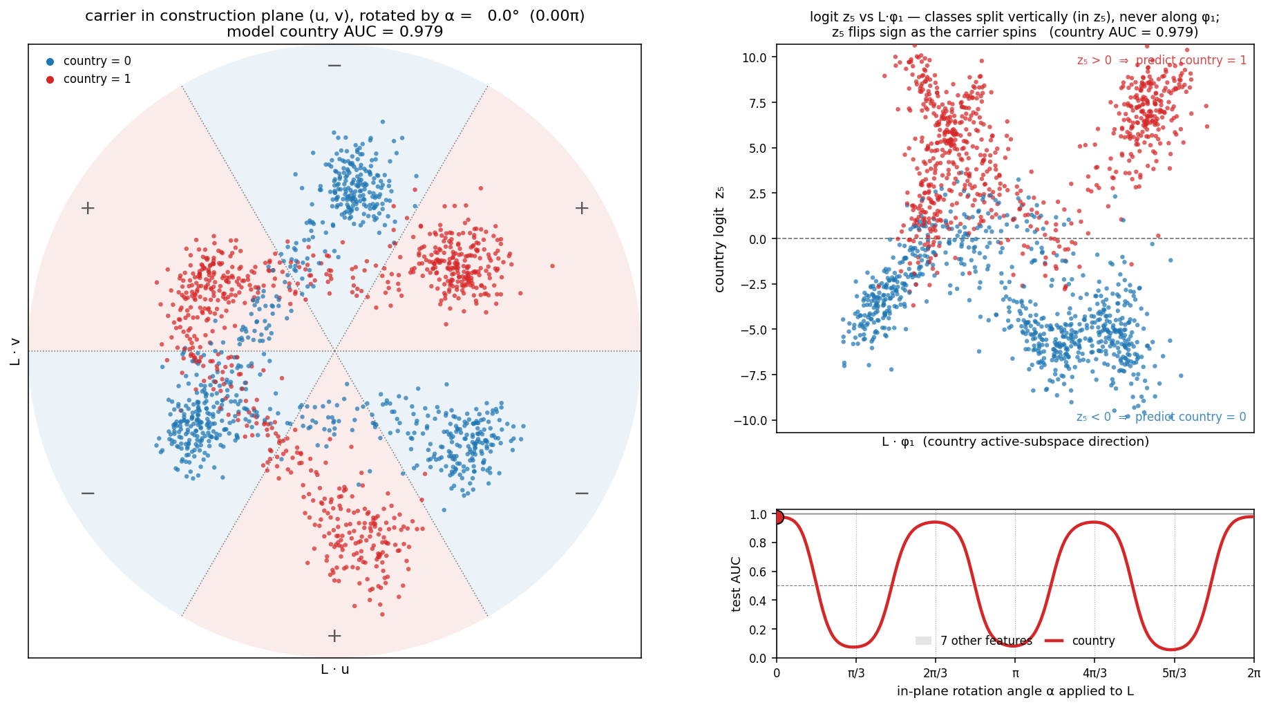
Left: The two-dimensional plan where the country feature is encoded in the classifier. The presence of this concept is approximately encoded as sign(sin 3θ). Six alternating blue and red wedges show the literal sign(sin 3θ) value, and the colored dots show the truth values. We rotate that plane by an angle, α, in a post-training step. Top-right: The model's country logit, z₅, plotted against the activations projected into the leading active subspace direction. Points above/below the dashed line are categorized by the network as country being present/absent, respectively. The points are colored by the true labels. Bottom-right: The resulting AUC of predicting the presence of the country concept for different rotations of the embedded pinwheel concept (swings with period 2π/3).

BlueDot Impact Technical AI Safety Puzzle #1

Problem Statement

The puzzle hands off a frozen all-MiniLM-L6-v2 sentence encoder and a tiny trained classifier (a 5-layer multilayer perceptron, 384→64→64→64→64→8). Pass a chunk of text through and, at a chosen intermediate layer, you get a 64-dimensional activation vector, L. The final layer of the classifier emits eight logits, which feed into sigmoid functions to become probabilities, one per text classification concept (i.e., does the text mention a number, a color, a country, a food, etc.).

Three questions are posed: (1) For which concept must the classifier do something nonlinear to L i.e., which one is not just a linear encoding? (2) What is the geometry of that nonlinear encoding? And (3) can you build a weirder representation of your own that is even harder to read out?

TASK 1

Which feature is nonlinear? Country.

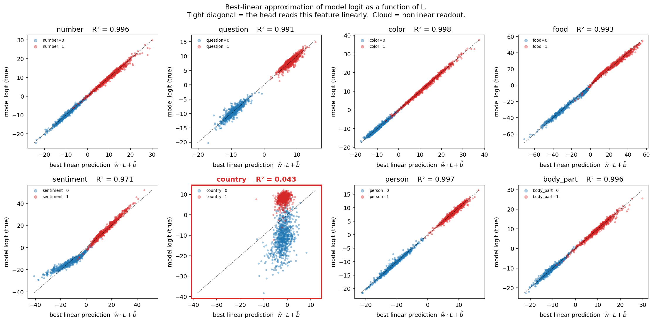
I fit a linear regression of each output logit onto L, and a logistic probe for each true label, training and scoring on the problem's provided train-test split. Seven features are essentially perfect lines: R² above 0.97, area under the curve (AUC) above 0.99. One is not. Country has a linear fit of R² = 0.043 and a best-linear-probe AUC of 0.47 in the held-out test data, which is below chance. However, a small multilayer perceptron recovers it from the very same activations at AUC 0.993. So I concluded that the country concept information is fully present in the activations; it's just not linearly decodable.

Eight-panel scatter of true model logit versus best linear prediction, one panel per feature. Seven panels fall on a tight diagonal; the country panel, highlighted in red, is a diffuse vertical cloud with R-squared 0.043.
Figure 1. Best-linear approximation of each feature's logit from L. Seven features sit on a tight diagonal. Country (highlighted, R² = 0.043) is a cloud: no linear function of L reproduces its logit.

TASK 2

The geometry: a gated, sign-flipped code

Why would a linear probe score <0.5 AUC in the test set below chance? To explore the structure, I borrowed a tool from classical model sensitivity analysis: active subspaces.

Primer · active subspaces

For a scalar function of many inputs (e.g., the country logit z₅ as a function of the 64-dimensional activation vector L) the active subspace (Constantine et al., 2014.) is the set of directions along which the output changes the most, on average. You find it by averaging the outer product of the gradient over the data and eigendecomposing the resulting square matrix, C = E[∇z₅ ∇z₅ᵀ]. The eigenvalues rank the directions by how strongly they move the logit, and the number of large ones is the effective dimensionality of the readout. A purely linear feature has exactly one active direction; country needs three to reach 99% of the variation, indicating that the readout is genuinely multi-directional.

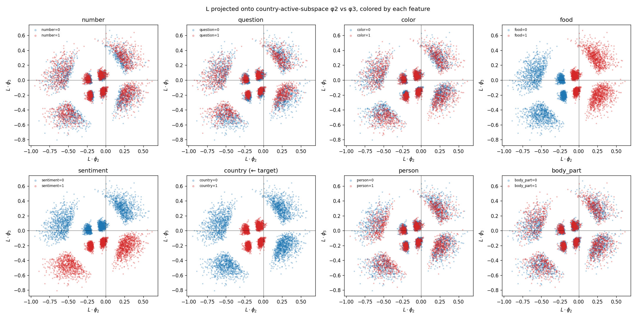
Projecting L onto the second and third of those directions (φ₂, φ₃) and coloring by each feature shows the gate directly: the country cloud resolves into discrete blobs, and lining the panels up reveals those blobs are sorted by food and sentiment.

Eight-panel scatter of L projected onto the second versus third country active-subspace eigenvectors, one panel per feature. The country panel shows compact central blobs; the food and sentiment panels show those same blobs split cleanly by color.
Figure 2. L projected onto the country active-subspace directions φ₂ (x) and φ₃ (y), colored by each feature. The country panel breaks into blobs; the food and sentiment panels split those same blobs cleanly by color — the two gates that select the readout direction.

If food and sentiment are the gates, then conditioning the probe on them should unlock the country feature. In Table 1, I recompute the AUC from Task 1 using a logistic regression conditional on these two features, splitting the data into four quadrants. I tested various feature pairs to see which pair best captured the country label.

Table 1: Country AUC for conditional probes. Data is split into four quadrants based on the binary values of the feature pair.
Feature PairCountry AUC (Conditional)
(food, sentiment) 0.989
(food, X) for X ∈ {question, person, number, body_part, color} 0.976–0.977
(sentiment, X) for X ∈ {number, body_part, question, color, person} 0.91
All pairs not involving food or sentiment 0.58–0.63

As shown in Table 1, pairing food and sentiment shoots the AUC up to 0.989. No other feature pair can close this gap. Food is the most important gate for resolving the sign of the computation, but sentiment is required to resolve the axis.

To investigate how these gates operate, I examined the cosine similarity between the linear directions found for each combination of the presence or absence of food and category. (This is a summary of the full derivation in the PDF.) The magnitude of the cosine similarity is approximately 1 only when food XOR sentiment agrees. The presence of the food concept flips the sign of the cosine similarity. We can thus deduce two rules: the linear combination of activations (A vs B) is set by food XOR sentiment, and the sign is set by food.

Table 2: Cosine similarities between the w vectors found in the logistic regressions, Pr(y₅) = σ(wjlj + b), for each quadrant of observed food and sentiment binary values.

cos(wi, wj) 0, 00, 11, 01, 1
0, 01.000.43−0.48−1.00
0, 10.431.00−0.99−0.46
1, 0−0.48−0.991.000.52
1, 1−1.00−0.460.521.00

index = (food, sentiment) · highlighted entries mark the same-axis pairs

This proved the model selects from two regression vectors (A and B) based on an XOR gate, and flips the sign based on the food category. This perfectly explains the below-chance AUC of 0.47 in Task 1: a global linear probe learns the orientation of the most populated quadrant, causing it to systematically misclassify the data in the sign-flipped quadrants.

Reconstructing the rule from conditional probes and the cosine structure of the per-quadrant readers gives a compact form:

w(food, sentiment) = (−1)food · A if food ⊕ sentiment = 0
                      (−1)food · B if food ⊕ sentiment = 1

The country direction is one of four sign-flipped vectors, +A, −A, +B, −B, with the sign set by food and the choice of axis (A vs B, about 60° apart) set by food XOR sentiment. A single global probe locks onto the most populated quadrant and is then systematically wrong in the sign-flipped ones, which is why we originally found a test AUC of 0.47. Conditioning the probe on the (food, sentiment) gates, decoded from L itself, lifts country from 0.47 to 0.989.

I verified the model truly uses this code, rather than merely admitting it, with a causal test: reflecting each activation across its own quadrant's reader hyperplane drives country from 0.994 to 0.026 (94% of predictions flip), while a reflection across a random orthogonal direction leaves it untouched. The sign-flip is load-bearing.
TASK 3

Building something weirder: the pinwheel

The provided model's code is a product of linear pieces, so a generic quadratic probe already cracks it (AUC 0.99). I wanted an encoding that fundamentally cannot be read by any conditional-linear or quadratic probe. So, I decided to suggest a phase encoder. Pick two orthonormal directions in L, project onto that plane to get an angle θ, and declare the country feature present exactly when sin 3θ > 0: six alternating wedges, like a pinwheel.

The class-conditional cloud is invariant under a 120° rotation, so its mean and covariance are identical for present and absent. There are no first- or second-degree probes that can tell them apart. The first monomial that separates the wedges is the cubic 3x²y − y³ = Im((x+iy)³). Running the full probe ladder on the trained pinwheel makes this concrete:

Table 3: Country AUC for a ladder of probes of increasing order, fit to the trained pinwheel phase encoding. The feature is fully present but cannot be read by anything below cubic order.
ProbeCountry AUC
Degree-1 logistic0.54
Conditional-linear (the encoding used in Task 2)0.64
Degree-2 logistic0.70
Degree-3 logistic0.97
The pinwheel model itself0.98

The feature is fully present and readable, but by nothing below cubic order. Getting a network to actually learn this took an information-bottleneck construction: the layers feeding the target are split into two independent channels so that country information exists nowhere in L except in the chosen plane, with a downstream phase bank of 24 half-cosine bumps warm-started around the circle. The finished model reads country at AUC 0.979 (within 1.5% of the original puzzle model).

For comparison, the original puzzle model's gated-linear encoding (a product of linear pieces) is easily captured by a generic quadratic probe (AUC 0.99). As Marvin Minsky and Seymour Papert noted in Perceptrons: An Introduction to Computational Geometry (Theorem 3.11, Chapter 3), the product of linear functionals can be learned by a quadratic classifier, which is exactly why we needed to push to a cubic phase code to build something genuinely weirder.

THE PROOF

Spin the plane, and the readout obeys

If country really is sign(sin 3θ), then rotating the carrier plane by an angle α adds α to every activation's phase, and the model's accuracy must move in a perfectly predictable way, with period 2π/3.

Crucially, this rotation is a purely post-training, post-processing step. The model's weights are entirely frozen. We intercept the 64-dimensional activation vector L right as it exits the target layer. We then isolate the specific 2D subspace (the uA, uB plane) that carries the country feature and apply a standard 2×2 rotation matrix R(α) to just that slice of the vector. The other 62 dimensions are left completely untouched. We then feed this surgically modified vector, L', into the rest of the frozen model.

Because the encoding depends entirely on the angle θ and not the radius, this rigid rotation perfectly shifts every point by α degrees around the center. Three snapshots from the animation above:

Rotation theta=0: country class points aligned with the readout wedges; logit cleanly separated; AUC 0.98
θ = 0  ·  AUC 0.98 aligned — readout correct
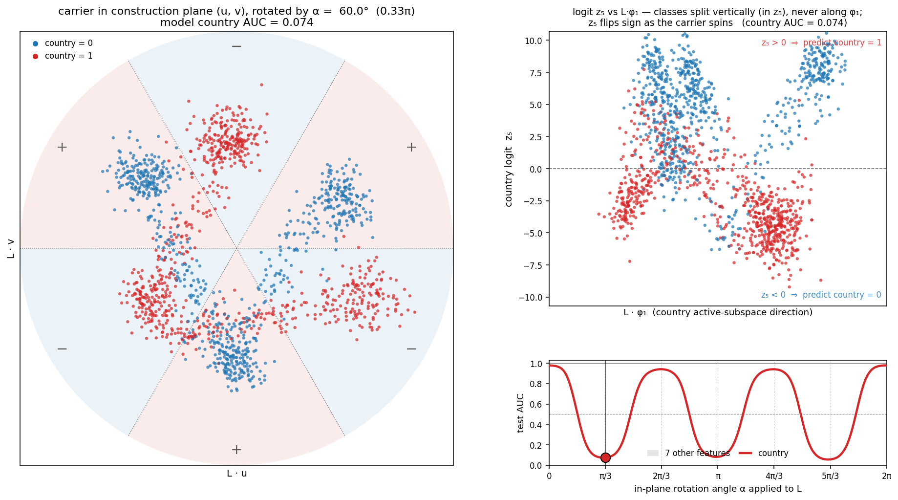
Rotation theta=pi/3: every point slides one wedge over into the opposite-parity sector; logit sign inverts; AUC 0.07
θ = π/3  ·  AUC 0.07 inverted — logit flips sign
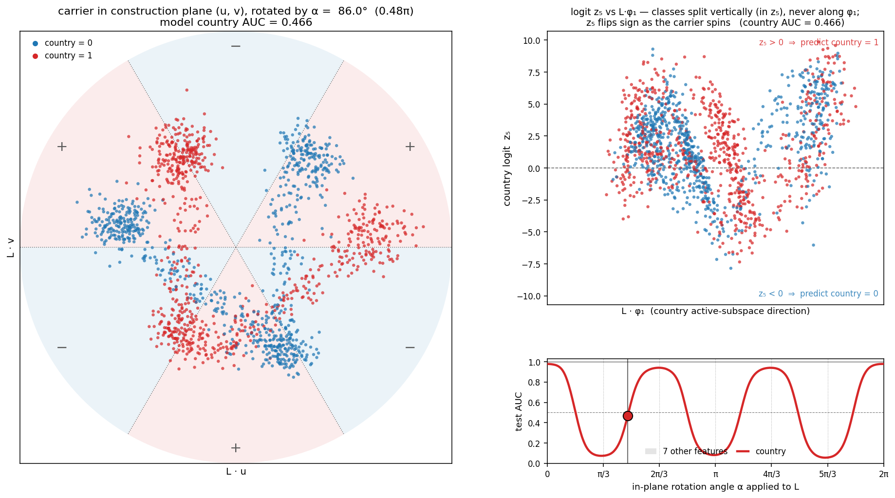
Rotation theta approximately pi/2: classes maximally mixed across the decision boundary; AUC about 0.47, chance
θ ≈ π/2  ·  AUC 0.47 crossover — pure chance
Figure 3. Snapshots of the pinwheel spin: rotating the (uA, uB) plane by α advances every activation's phase by the same amount, so the country readout slides from correct at θ = 0, through a one-wedge sign inversion at θ = π/3, to pure chance where the classes cross near θ ≈ π/2.

At θ = 0 the class colors match their wedges and the country logit z₅ sits cleanly above and below its decision boundary. At θ = π/3 every point has slid exactly one wedge over into the opposite-parity sector: the logit flips sign and accuracy collapses to 0.07. Pass through θ ≈ π/2 and the two classes are maximally mixed at pure chance, 0.47. Keep going to θ = 2π/3 and country snaps back to 0.94. Throughout, scaling the radius does nothing (the code is in the angle, not the magnitude) and the other seven features never drop below 0.996. The phase encoding is exactly what the model uses.

WHY IT MATTERS

Probes have a reading level

A linear probe that returns chance is not proof that a concept is absent. It can instead mean that the concept is written in a basis the probe cannot read. The newly-included country feature is below-chance to a line, mild to a quadratic, and obvious to a cubic. For interpretability and for auditing, the lesson is that negative probe results are conditional on the probe's expressivity. The honest move is to state the ladder you searched and, when you can, to verify causally by intervening on the representation itself rather than trusting a fitted readout.

REFERENCES

References

  1. Constantine, P. G., Dow, E., & Wang, Q. (2014). Active subspace methods in theory and practice: applications to kriging surfaces. SIAM Journal on Scientific Computing, 36(4), A1500-A1524.
  2. Belrose, N., Schneider-Joseph, D., Ravfogel, S., Cotterell, R., Raff, E., & Biderman, S. (2023). Leace: Perfect linear concept erasure in closed form. Advances in Neural Information Processing Systems, 36, 66044-66063.
  3. Minsky, M., & Papert, S. (1969). Perceptrons: An Introduction To Computational Geometry. The MIT Press. (See Theorem 3.11 in Chapter 3).

Code and the rotation/reflection causal suite available on request.